13장 요약정리
2. 파이토치의 계산 그래프
- 파이토치는 유향 비순환그래프를 기반으로 계산 수행
2.1. 계산 그래프 이해
- 파이토치는 계산 그래프에 크게 의존함 => 계산 그래프를 사요하여 입력에서 출력까지 텐서 간의 관계 유도함.
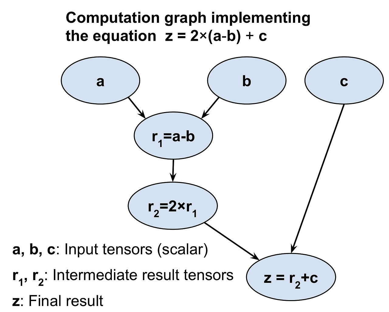
---> 파이토치는 계산 그래프를 구성하고 이를 사용하여 그레이디언트 계산함.
3. 모델 파라미터를 저장하고 업데이트하기 위한 파이토치 텐서 객체
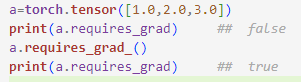
- 파이토치에서는 그레이디언트를 계산해야 하는 특수한 텐서 객체를 사용하여 훈련 중에 모델의 파라미터를 저장하고 업데이트할 수 있음. ==> 특수한 텐서 객체는 사용자가 지정한 초깃값 다음에 require_grad를 True로 지정하면 생성 가능함. ==> 현재 부동소수점 텐서 및 복소수 dtype의 텐서만 그레이디언트를 요구할 수 있음.
1 2 3 4 | a=torch.tensor(3.14,requires_grad=True) print(a) b=torch.tensor([1.0,2.0,3.0],requires_grad=True) print(b) | cs |
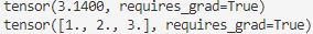
--> requires_grad 기본값은 False임. requires_grad() 메서드를 호출하여 True로 설정할 수 있음.
- 신경망 모델은 역전파하는 동안 대칭성을 깨기 위해 파라미터를 랜덤한 가중치로 초기화 해야함. => 그렇지 않으면 다층 신경망이 로지스틱 회귀같은 단일층 신경망보다 더 유용하지 않기 때문임. => 파이토치는 다양한 확률 분포를 기반으로 난수를 생성할 수 있음!
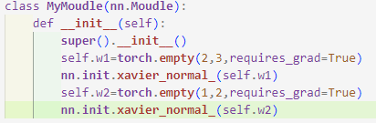
<글로럿 초기화로 텐서 만들기>
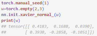
--> 더 실용적인 예
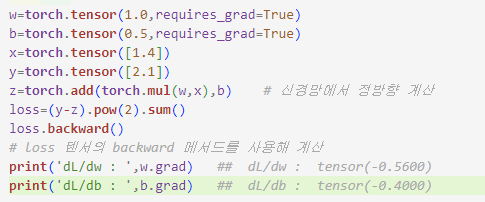
4. 자동 미분으로 그레이디언트 계산
--> 신경망을 최적화하려면 신경망의 가중치에 대한 비용의 그레이디언트를 계산해야함.
4.1. 훈련 가능한 변수에 대한 손실의 그레이디언트 계산
- 파이토치는 자동미분 지원 => 중첩된 함수의 그레이디언트를 계산하기 위한 연쇄 법칙을 구현한 것.
- 어떤 출력이나 중간 텐서를 만드는 일련의 연산을 정의할 때 파이토치는 계산 그래프 안에서 의존성을 가지는 노드에 대해 이런 텐서의 그레이디언트를 계산하는 기능 지원. => torch.autograd 모듈의 backward 메서드를 호출하여 그레이디언트 계산. => 그래프의 마지막노드에 대해 주어진 텐서의 그레이디언트 합을 계산
4.2. 자동 미분 이해하기
- 자동미분
- 특정 산술 연산의 그레이디언트를 계산하기 위한 일련의 컴퓨팅 기술
- (일련의 연산으로 표현된) 어던 계산의 그레이디언트는 연쇄 법칙을 반복적으로 적용하여 얻은 그레이디언트를 누적하여 구함.
- 자동미분은 전진 모드, 후진 모드 방법으로 계산할 수 있는 데 파이토치는 역전파 구현에 더 효율적인 후진 모드 자동미분을 사용함.
5. torch.nn 모듈을 사용하여 일반적인 아키텍처 구현하기
5.1. nn.Sequential 기반의 모델 구현하기
--> nn.Sequential에서 모델 안의 층은 순서대로 연결됨.
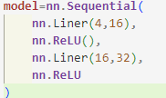
---> 첫번째 완전 연결 층의 출력이 첫번째 ReLU 층의 입력으로 사용됨.
---> 두번째 완전 연결 층의 출력은 두 번째 ReLU 층의 입력으로 사용됨.
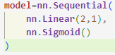
5.2. 손실 함수 선택하기
--> 손실 함수 선택은 문제에 따라 다름. (ex 크로스 엔트로피 손실함수: 분류 작업에 사용)
--> 최적화 알고리즘 중에서는 SGD와 Adam이 가장 널리 사용되는 방법.
5.3. XOR 분류 문제
① 데이터셋 생성
- [-1,1) 사이의 균등 분포에서 뽑은 두개의 특성을 가진 200개의 훈련 샘플이 들어 있는 작은 데이터셋 생성
② 규칙에 따라 훈련샘플 i에 정답 레이블 부여
1 2 3 4 5 6 7 8 9 10 11 12 13 | torch.manual_seed(1) np.random.seed(1) x=np.random.uniform(low=-1,high=1,size=(200,2)) # 데이터 생성 y=np.ones(len(x)) # 레이블 생성 y[x[:,0]*x[:,1]<0]=0 n_train=100 # 훈련데이터와 검증 데이터 분리 x_train=torch.tensor(x[:n_train,:],dtype=torch.float32) y_train = torch.tensor(y[:n_train], dtype=torch.float32) x_valid = torch.tensor(x[n_train:, :], dtype=torch.float32) y_valid = torch.tensor(y[n_train:], dtype=torch.float32) | cs |
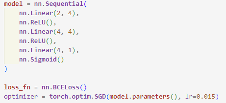
③ 모델 정의
- 층이 많을 수록 각 층에 뉴런 개수가 만흘수록 모델의 수용능력(모델이 얼마나 복잡한 함수를 근사할 수 있는지를 측정한 것)이 큼.
- 많은 파라미터를 가지고 있으면 모델이 복잡한 함수를 근사할 수 있지만 모델이 클수록 훈련하기 힘듦.
④ 손실함수와 옵티마이저 초기화

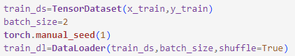
⑤ 훈련 데이터의 배치 크기가 2인 데이터 로더 생성
⑥ 훈련
1 2 3 4 5 6 7 8 9 10 11 12 13 14 15 16 17 18 19 20 21 22 23 24 25 26 27 28 | torch.manual_seed(1) num_epochs=200 def train(model,num_epochs,train_dl,x_valid,y_vaild): loss_hist_train=[0]*num_epochs accuracy_hist_train=[0]*num_epochs loss_hist_valid=[0]*num_epochs accuracy_hist_vaild=[0]*num_epochs for epoch in range(num_epochs): for x_batch,y_batch in train_dl: pred=model(x_batch)[:,0] loss=loss_fn(pred,y_batch) loss.backward() optimizer.step() optimizer.zero_grad() loss_hist_train[epoch]+=loss.item() is_correct=((pred>=0.5).float()==y_batch).float() accuracy_hist_train[epoch]+=is_correct.mean() loss_hist_train[epoch]/=n_train/batch_size accuracy_hist_train[epoch]/=n_train/batch_size pred=model(x_valid)[:,0] loss=loss_fn(pred,y_vaild) loss_hist_valid[epoch]=loss.item() is_correct=((pred>=0.5).float()==y_vaild).float() accuracy_hist_vaild[epoch]+=is_correct.mean() return loss_hist_train,loss_hist_valid,\ accuracy_hist_train,accuracy_hist_vaild history=train(model,num_epochs,train_dl,x_valid,y_valid) | cs |
⑦ 그래프
1 2 3 4 5 6 7 8 9 10 11 12 13 14 | fig = plt.figure(figsize=(16, 4)) ax = fig.add_subplot(1, 2, 1) plt.plot(history[0], lw=4) plt.plot(history[1], lw=4) plt.legend(['Train loss', 'Validation loss'], fontsize=15) ax.set_xlabel('Epochs', size=15) ax = fig.add_subplot(1, 2, 2) plt.plot(history[2], lw=4) plt.plot(history[3], lw=4) plt.legend(['Train acc.', 'Validation acc.'], fontsize=15) ax.set_xlabel('Epochs', size=15) plt.show() | cs |
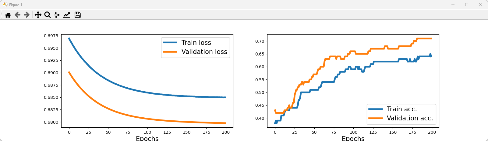
--> 결과에서 볼 수 있듯이 은닉층이 없는 간단한 모델은 선형결정 경계만 찾을 수 있음(XOR 문제 풀 수 없음)
=> 이로 인해 훈련 데이터셋과 검증 데이터셋의 손실이 매우 높고 분류 정확도는 매우 낮음.
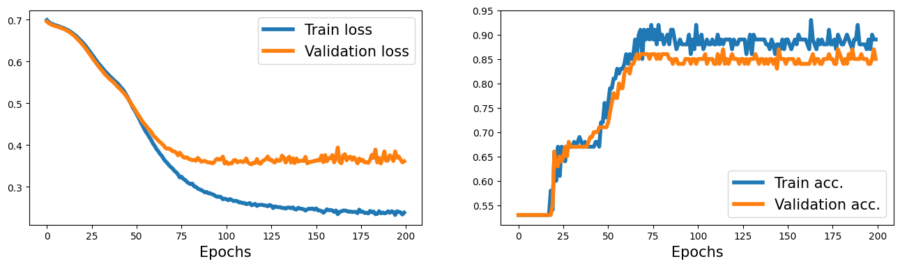
- 일반 근사 이론: 하나의 은닉층과 매우 많은 은닉 유닛을 가진 피드포워드 신경망은 임의의 연속 함수를 비교적 잘 근사할 수 있음.
<XOR 문제를 만족스럽게 해결하는 방법>
1. 은닉층을 추가하고 검증 데이터셋에서 만족스러운 결과가 나올 때까지 은닉 유닛 개수를 바꾸면서 비교해보는 것.
--> 은닉 유닛을 늘린다는 것은 층의 폭을 넓히는 것과 같음.
2. 더 많은 은닉층을 추가하여 모델의 깊이를 깊게 하는것.
---> 네트워크의 폭 대신 깊이를 깊게 하면 모델 수용 능력을 달성하는 데 필요한 파라미터 개수가 적다는 장점이 있지만 넓은 모델에 비해 깊은 모델은 그레이디언트가 폭주하거나 소멸될 수 있어 훈련하기 어렵다는 단점이 있음.
5.4. nn.Moudle로 유연성이 높은 모델 만들기
--> 복잡한 모델은 만드는 또 다른 방법은 nn.Moudle 클래스를 상속하는 것이다!
1 2 3 4 5 6 7 8 9 10 11 12 13 14 15 16 17 18 19 | # nn.Moudle 클래스를 상속한 새로운 클래스 만들기 class MyMoudle(nn.Module): # 생성자 메서드 정의 def __init__(self): super().__init__() # 층층 l1=nn.Linear2,4) a1=nn.ReLU() l2=nn.Linear(4,4) a2=nn.ReLU() l3=nn.Linear(4,1) a3=nn.Sigmoid() l=[l1,a1,l2,a2,l3,a3] # 모든 층 nn.ModuleList 객체에 넣음 self.moudle_list=nn.ModuleList(l) # forward() 메서드를 사용하여 정방향 계산 정의 def forward(self,x): for f in self.moudle_list: x=f(x) return x | cs |
5.5. 파이토치에서 사용자 정의 층 만들기
- 파이토치에서 제공하지 않는 층을 새로 정의해야 하는 경우 nn.Module 클래스를 상속하여 새로운 클래스를 정의할 수 있음.
1 2 3 4 5 6 7 8 9 10 11 12 13 14 15 16 17 18 19 20 21 | # nn.Module 클래스 상속 class NoisyLinear(nn.Module): # 생성자 # input_size: 변수를 만들고 초기화 할 수 있음, 변수 생성을 지연하고 다른 메서드에 변수 생성을 위임할 수 있음 def __init__(self,input_size,output_size, noise_stddev=0.1): super().__init__() w=torch.Tensor(input_size,output_size) self.w=nn.Parameter(w) b=torch.Tensor(output_size).fill_(0) self.b=nn.Parameter(b) self.noise_stddev=noise_stddev # training : 층이 훈련에 사용되는지 추론에 사용되는지 구분하는 매개변수 def forward(self,x,training=False): if training: noise=torch.normal(0.0,self.noise_stddev,x.shape) x_new=torch.add(x,noise) else: x_new=x return torch.add(torch.mm(x_new,self.w),self.b) | cs |
--> NoisyLinear 층을 다층 퍼셉트론의 첫번째 은닉층으로 사용함.
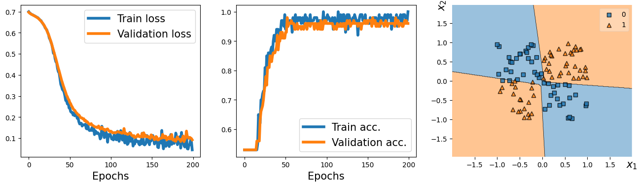
1 2 3 4 5 6 7 8 9 10 11 12 13 14 15 16 17 18 19 20 21 22 23 24 25 26 27 28 29 30 31 32 33 34 35 36 37 38 39 40 41 42 43 44 45 46 47 48 49 50 51 52 53 54 55 56 57 58 59 60 61 62 63 64 65 66 67 68 69 70 71 72 73 74 75 76 77 78 79 80 81 82 83 84 85 86 87 88 89 90 91 92 93 94 95 96 97 98 99 100 101 102 103 104 105 106 107 108 109 110 111 112 113 114 115 116 117 118 119 120 121 122 123 124 125 126 127 128 129 | from torch.utils.data import DataLoader,TensorDataset from mlxtend.plotting import plot_decision_regions import torchvision.transforms as transforms import numpy as np import torch.nn as nn import matplotlib.pyplot as plt import torch np.random.seed(1) torch.manual_seed(1) x = np.random.uniform(low=-1, high=1, size=(200, 2)) y = np.ones(len(x)) y[x[:, 0] * x[:, 1]<0] = 0 n_train = 100 x_train = torch.tensor(x[:n_train, :], dtype=torch.float32) y_train = torch.tensor(y[:n_train], dtype=torch.float32) x_valid = torch.tensor(x[n_train:, :], dtype=torch.float32) y_valid = torch.tensor(y[n_train:], dtype=torch.float32) train_ds = TensorDataset(x_train, y_train) batch_size = 2 torch.manual_seed(1) train_dl = DataLoader(train_ds, batch_size, shuffle=True) # nn.Module 클래스 상속 class NoisyLinear(nn.Module): # 생성자 # input_size: 변수를 만들고 초기화 할 수 있음, 변수 생성을 지연하고 다른 메서드에 변수 생성을 위임할 수 있음 def __init__(self,input_size,output_size, noise_stddev=0.1): super().__init__() w=torch.Tensor(input_size,output_size) self.w=nn.Parameter(w) b=torch.Tensor(output_size).fill_(0) self.b=nn.Parameter(b) self.noise_stddev=noise_stddev # training : 층이 훈련에 사용되는지 추론에 사용되는지 구분하는 매개변수 def forward(self,x,training=False): if training: noise=torch.normal(0.0,self.noise_stddev,x.shape) x_new=torch.add(x,noise) else: x_new=x return torch.add(torch.mm(x_new,self.w),self.b) # MyNoisyModule 클래스 class MyNoisyModule(nn.Module): def __init__(self): super().__init__() self.l1 = NoisyLinear(2, 4, 0.07) # 첫번째 은닉층 NoisyLinear로 사용 self.a1 = nn.ReLU() self.l2 = nn.Linear(4, 4) self.a2 = nn.ReLU() self.l3 = nn.Linear(4, 1) self.a3 = nn.Sigmoid() def forward(self, x, training=False): x = self.l1(x, training) x = self.a1(x) x = self.l2(x) x = self.a2(x) x = self.l3(x) x = self.a3(x) return x def predict(self, x): x = torch.tensor(x, dtype=torch.float32) pred = self.forward(x)[:, 0] return (pred>=0.5).float() torch.manual_seed(1) model = MyNoisyModule() loss_fn = nn.BCELoss() optimizer = torch.optim.SGD(model.parameters(), lr=0.015) torch.manual_seed(1) num_epochs = 200 loss_hist_train = [0] * num_epochs accuracy_hist_train = [0] * num_epochs loss_hist_valid = [0] * num_epochs accuracy_hist_valid = [0] * num_epochs for epoch in range(num_epochs): for x_batch, y_batch in train_dl: pred = model(x_batch, True)[:, 0] # 훈련배치에 대한 예측 loss = loss_fn(pred, y_batch) loss.backward() optimizer.step() optimizer.zero_grad() loss_hist_train[epoch] += loss.item() is_correct = ((pred>=0.5).float() == y_batch).float() accuracy_hist_train[epoch] += is_correct.mean() loss_hist_train[epoch] /= n_train/batch_size accuracy_hist_train[epoch] /= n_train/batch_size pred = model(x_valid)[:, 0] loss = loss_fn(pred, y_valid) loss_hist_valid[epoch] = loss.item() is_correct = ((pred>=0.5).float() == y_valid).float() accuracy_hist_valid[epoch] += is_correct.mean() fig = plt.figure(figsize=(16, 4)) ax = fig.add_subplot(1, 3, 1) plt.plot(loss_hist_train, lw=4) plt.plot(loss_hist_valid, lw=4) plt.legend(['Train loss', 'Validation loss'], fontsize=15) ax.set_xlabel('Epochs', size=15) ax = fig.add_subplot(1, 3, 2) plt.plot(accuracy_hist_train, lw=4) plt.plot(accuracy_hist_valid, lw=4) plt.legend(['Train acc.', 'Validation acc.'], fontsize=15) ax.set_xlabel('Epochs', size=15) ax = fig.add_subplot(1, 3, 3) plot_decision_regions(X=x_valid.numpy(), y=y_valid.numpy().astype(np.int64), clf=model) ax.set_xlabel(r'$x_1$', size=15) ax.xaxis.set_label_coords(1, -0.025) ax.set_ylabel(r'$x_2$', size=15) ax.yaxis.set_label_coords(-0.025, 1) #plt.savefig('figures/13_06.png', dpi=300) plt.show() | cs |
8. 고수준 파이토치 API: 파이토치 라이트닝 소개
- 파이토치 라이트닝
- 반복적인 코드의 대부부을 제거함으로써 심층 신경망을 더 간단하게 훈련할 수 있음.
- 단순성과 유연성에 중점을 두고 있지만 멀티 GPU 지원 및 낮은 정밀도의 고속 훈련과 같은 많은 고급 기능도 사용할 수 있음.
8.1. 파이토치 라이트닝 모델 준비하기
- LightningModule 사용 ==> pip install pytorch-lightning
1 2 3 4 5 6 7 8 9 10 11 12 13 14 15 16 17 18 19 20 21 22 23 24 25 26 27 28 29 30 31 32 33 34 35 36 37 38 39 40 41 42 43 44 45 46 47 48 49 50 51 52 53 54 55 56 57 58 59 60 61 62 63 64 65 66 67 68 69 70 71 72 73 74 75 76 77 | import pytorch_lightning as pl import torch import torch.nn as nn from torchmetrics import __version__ as torchmetrics_version from pkg_resources import parse_version from torchmetrics import Accuracy class MultiLayerPerceptron(pl.LightningModule): # 생성자 def __init__(self, image_shape=(1, 28, 28), hidden_units=(32, 16)): super().__init__() # PL 속성: # 정확도 속성 추가 self.train_acc = Accuracy(task="multiclass", num_classes=10) self.valid_acc = Accuracy(task="multiclass", num_classes=10) self.test_acc = Accuracy(task="multiclass", num_classes=10) # 이전 코드와 비슷한 모델: input_size = image_shape[0] * image_shape[1] * image_shape[2] all_layers = [nn.Flatten()] for hidden_unit in hidden_units: layer = nn.Linear(input_size, hidden_unit) all_layers.append(layer) all_layers.append(nn.ReLU()) input_size = hidden_unit all_layers.append(nn.Linear(hidden_units[-1], 10)) self.model = nn.Sequential(*all_layers) # 입력데이터로 모델을 호출할 때 로짓을 반환하는 간단한 정방향 계산 구현 # 로짓: 네트워크에서 소프트맥스 층 전에 있는 마지막 완전 연결 층의 출력 def forward(self, x): x = self.model(x) return x # 이 로짓은 다음에 설명할 훈련, 검증 및 테스트 단계에 사용됨 def training_step(self, batch, batch_idx): x, y = batch logits = self(x) loss = nn.functional.cross_entropy(logits, y) preds = torch.argmax(logits, dim=1) self.train_acc.update(preds, y) self.log("train_loss", loss, prog_bar=True) return loss def on_train_epoch_end(self): self.log("train_acc", self.train_acc.compute()) self.train_acc.reset() def validation_step(self, batch, batch_idx): x, y = batch logits = self(x) loss = nn.functional.cross_entropy(logits, y) preds = torch.argmax(logits, dim=1) self.valid_acc.update(preds, y) self.log("valid_loss", loss, prog_bar=True) return loss def on_validation_epoch_end(self): self.log("valid_acc", self.valid_acc.compute(), prog_bar=True) self.valid_acc.reset() def test_step(self, batch, batch_idx): x, y = batch logits = self(x) loss = nn.functional.cross_entropy(logits, y) preds = torch.argmax(logits, dim=1) self.test_acc.update(preds, y) self.log("test_loss", loss, prog_bar=True) self.log("test_acc", self.test_acc.compute(), prog_bar=True) return loss def configure_optimizers(self): optimizer = torch.optim.Adam(self.parameters(), lr=0.001) return optimizer | cs |
- training_step 메서드
- 훈련 중에 한번의 정방향 계산을 정의하며, 정확도와 손실을 추적하여 나중에 분석할 수 있음.
- 훈련 중 각 개별 배치에 대해 실행됨.
- on_train_epoch_end 메서드
- 훈련 에포크가 끝날 때마다 실행
- 훈련 과정에서 누적된 정확도 값으로 훈련 세트 정확도 계산
- validation_step, test_step
- 검증과 테스트 평가 과정 정의
- 단일 배치를 받으므로 torchmetric의 Accuracy에 정확도 기록
- configure_optimizers 메서드
- 훈련에 사용할 옵티마이저 지정
8.2. 라이트닝을 위한 데이터 로더 준비하기
1 2 3 4 5 6 7 8 9 10 11 12 13 14 15 16 17 18 19 20 21 22 23 24 25 26 27 28 29 30 31 32 33 34 35 36 37 38 39 40 41 42 43 44 45 46 47 48 | from torch.utils.data import DataLoader from torch.utils.data import random_split from torchvision.datasets import MNIST from torchvision import transforms class MnistDataModule(pl.LightningDataModule): def __init__(self, data_path='./'): super().__init__() self.data_path = data_path self.transform = transforms.Compose([transforms.ToTensor()]) # 데이터셋 다운로드와 같은 일반적인 단계 정의 def prepare_data(self): MNIST(root=self.data_path, download=True) # 훈련, 검증 및 테스트에 사용되는 데이터셋 정의 def setup(self, stage=None): # stage는 'fit', 'validate', 'test', 'predict' 중 하나입니다. mnist_all = MNIST( root=self.data_path, train=True, transform=self.transform, download=False ) self.train, self.val = random_split( mnist_all, [55000, 5000], generator=torch.Generator().manual_seed(1) ) self.test = MNIST( root=self.data_path, train=False, transform=self.transform, download=False ) def train_dataloader(self): return DataLoader(self.train, batch_size=64, num_workers=2) def val_dataloader(self): return DataLoader(self.val, batch_size=64, num_workers=2) def test_dataloader(self): return DataLoader(self.test, batch_size=64, num_workers=2) torch.manual_seed(1) mnist_dm = MnistDataModule() | cs |
8.3. 라이트닝 Trainer 클래스를 사용하여 모델 훈련하기
1 2 3 4 5 6 7 8 9 10 11 12 13 | from pytorch_lightning.callbacks import ModelCheckpoint mnistclassifier = MultiLayerPerceptron() callbacks = [ModelCheckpoint(save_top_k=1, mode='max', monitor="valid_acc")] # 가장 높은 성능의 모델 저장하기 if torch.cuda.is_available(): # GPU를 가지고 있다면 trainer = pl.Trainer(max_epochs=10, callbacks=callbacks, gpus=1) else: trainer = pl.Trainer(max_epochs=10, callbacks=callbacks) trainer.fit(model=mnistclassifier, datamodule=mnist_dm) | cs |
- 라이트닝은 Trainer 클래스를 구현하여 zero_grad(), backward(), optimizer.step() 호출과 같은 모든 중간 단계를 대신 처리함으로써 매우 편리하게 모델을 훈련할 수 있음
- 하나 이상의 GPU를 쉽게 지정할 수 있음.
8.4. 텐서보드로 모델 평가하기
- 라이트닝은 lightning_logs라는 하위 폴더에서훈련 기록을 저장함. => 훈련 실행을 시각화하기 위해 명령줄 터미널에서 tensorboard --logdir lightning_logs/를 실행하면 웹 브라우저에서 텐서보드가 열림.
1 2 3 4 5 6 7 8 9 10 11 12 13 14 15 16 17 18 19 20 21 22 23 24 25 26 27 28 29 30 31 32 33 34 35 36 37 38 39 40 41 42 43 44 45 46 47 48 49 50 51 52 53 54 55 56 57 58 59 60 61 62 63 64 65 66 67 68 69 70 71 72 73 74 75 76 77 78 79 80 81 82 83 84 85 86 87 88 89 90 91 92 93 94 95 96 97 98 99 100 101 102 103 104 105 106 107 108 109 110 111 112 113 114 115 116 117 118 119 120 121 122 123 124 125 126 127 128 129 130 131 132 133 134 135 136 137 138 139 140 141 142 | import torch import pytorch_lightning as pl import torch.nn as nn from torchmetrics import Accuracy from torch.utils.data import DataLoader from torch.utils.data import random_split from torchvision.datasets import MNIST from torchvision import transforms from pytorch_lightning.callbacks import ModelCheckpoint class MultiLayerPerceptron(pl.LightningModule): def __init__(self, image_shape=(1, 28, 28), hidden_units=(31, 26)): super().__init__() self.train_acc = Accuracy(task="multiclass", num_classes=10) # 정확도 속성 -> 훈련 중에 정확도를 추적할 수 있음 self.valid_acc = Accuracy(task="multiclass", num_classes=10) # torchmetrics에 속함 self.test_acc = Accuracy(task="multiclass", num_classes=10) input_size = image_shape[0] * image_shape[1] * image_shape[2] all_layers = [nn.Flatten()] for hidden_unit in hidden_units: layer = nn.Linear(input_size, hidden_unit) all_layers.append(layer) all_layers.append(nn.ReLU()) input_size = hidden_unit all_layers.append(nn.Linear(hidden_units[-1], 10)) self.model = nn.Sequential(*all_layers) def forward(self, x): # 입력 데이터로 모델을 호출할 때 마지막 완전 연결층의 출력을 반환하는 계산 수행 x = self.model(x) return x def training_step(self, batch, batch_idx): x, y = batch logits = self(x) loss = nn.functional.cross_entropy(self(x), y) preds = torch.argmax(logits, dim=1) # 줄일 차원 1 self.train_acc.update(preds, y) self.log("train_loss", loss, prog_bar=True) return loss def on_train_epoch_end(self): self.log("train_acc", self.train_acc.compute()) self.train_acc.reset() def validation_step(self, batch, batch_idx): x, y = batch logits = self(x) loss = nn.functional.cross_entropy(self(x), y) preds = torch.argmax(logits, dim=1) self.valid_acc.update(preds, y) self.log("valid_loss", loss, prog_bar=True) return loss def on_validation_epoch_end(self): self.log("valid_acc", self.valid_acc.compute(), prog_bar=True) self.valid_acc.reset() def test_step(self, batch, batch_idx): x, y = batch logits = self(x) loss = nn.functional.cross_entropy(self(x), y) preds = torch.argmax(logits, dim=1) self.test_acc.update(preds, y) self.log("test_loss", loss, prog_bar=True) self.log("test_acc", self.test_acc.compute(), prog_bar=True) return loss def configure_optimizers(self): optimizer = torch.optim.Adam(self.parameters(), lr=0.001) return optimizer class MnistDataModule(pl.LightningDataModule): def __init__(self, data_path='./'): super().__init__() self.data_path = data_path self.transform = transforms.Compose([transforms.ToTensor()]) def prepare_data(self): MNIST(root=self.data_path, download=True) def setup(self, stage=None): mnist_all = MNIST( root=self.data_path, train=True, transform=self.transform, download=False ) self.train, self.val = random_split( mnist_all, [55000, 5000], generator=torch.Generator().manual_seed(1) ) self.test = MNIST( root=self.data_path, train=False, transform=self.transform, download=False ) def train_dataloader(self): return DataLoader(self.train, batch_size=64, num_workers=4) def val_dataloader(self): return DataLoader(self.val, batch_size=64, num_workers=4) def test_dataloader(self): return DataLoader(self.test, batch_size=64, num_workers=4) import torch.multiprocessing if __name__=='__main__': # 오류땜에 추가 import os log_dir = './lightning_logs' if os.path.exists(log_dir) and not os.path.isdir(log_dir): os.remove(log_dir) # 기존 파일 삭제 os.makedirs(log_dir, exist_ok=True) # 디렉토리 생성 torch.multiprocessing.freeze_support() torch.manual_seed(1) mnist_dm = MnistDataModule() mnistclassifier = MultiLayerPerceptron() callbacks = [ModelCheckpoint(save_top_k=1, mode='max', monitor="valid_acc")] if torch.cuda.is_available(): # if you have GPUs trainer = pl.Trainer(max_epochs=15, callbacks=callbacks, gpus=1) else: trainer = pl.Trainer(max_epochs=15, callbacks=callbacks) trainer.fit(model=mnistclassifier, datamodule=mnist_dm) | cs |
13장 정리문제
1) 훈련과 검증의 차이를 설명하라. 검증이 왜 필요한지 설명하고 훈련로스와 검증로스를 이용하여 과적합을 판단하는 방법을 설명하라.
- 훈련은 데이터를 이용해서 모델의 가중치와 파라미터를 최적화하는 과정이고 검증은 최적화된 파라미터를 사용해서 모델의 성능을 평가하는 과정이다.
- 검증 과정에서 모델이 새로운 데이터에 대해 얼마나 잘 일반화 할 수 있는지 판단할 수 있고 훈련 데이터에만 과도하게 적응하는 경우(과적합) 테스트 데이터에서 성능이 저하될 수 있는데 이러한 문제를 검증 과정에서 감지할 수 있기 때문에 필요하다.
- 훈련 로스와 검증로스가 함께 감소하면서 유사한 값을 유지하는 경우는 좋은학습이고, 훈련 로스는 계속 감소하지만 검증 로스가 어느 순간부터 증가하는 경우 과적합이다.
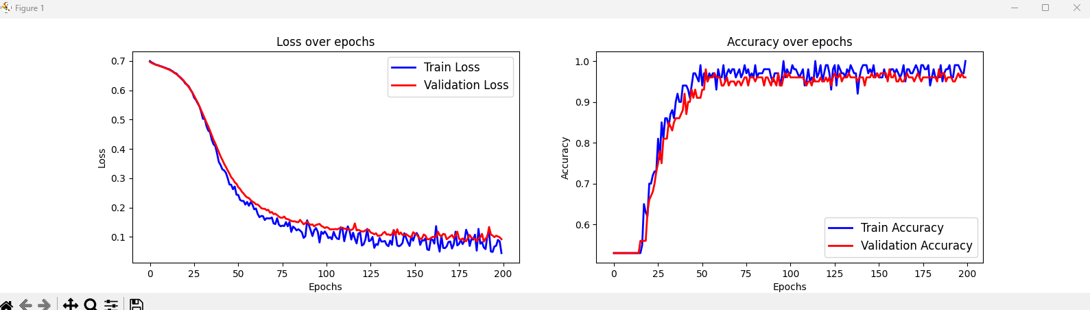
2) 신경망의 훈련예제에서 훈련/검증 손실과 정확도를 그래프로 그리는 방법을 설명하라.
- 매 에퍽마다 실시간으로 그래프를 업데이트하도록 할것 -> 훈련동안 시간의 흐름에 따라 loss의 변화를 확인가능하도록 할것
1 2 3 4 5 6 7 8 9 10 11 12 13 14 15 16 17 18 19 20 21 22 23 24 25 26 27 28 29 30 31 32 33 34 35 36 37 38 39 40 41 42 43 44 45 46 47 48 49 50 51 52 53 54 55 56 57 58 59 60 61 62 63 64 65 66 67 68 69 70 71 72 73 74 75 76 77 78 79 80 81 82 83 84 85 86 87 88 89 90 91 92 93 94 95 96 97 98 99 100 101 102 103 104 105 106 107 108 109 110 111 112 113 114 115 116 117 118 119 120 121 122 123 124 125 126 127 128 129 130 131 | from torch.utils.data import DataLoader,TensorDataset from mlxtend.plotting import plot_decision_regions import torchvision.transforms as transforms import numpy as np import torch.nn as nn import matplotlib.pyplot as plt import torch np.random.seed(1) torch.manual_seed(1) x = np.random.uniform(low=-1, high=1, size=(200, 2)) y = np.ones(len(x)) y[x[:, 0] * x[:, 1]<0] = 0 n_train = 100 x_train = torch.tensor(x[:n_train, :], dtype=torch.float32) y_train = torch.tensor(y[:n_train], dtype=torch.float32) x_valid = torch.tensor(x[n_train:, :], dtype=torch.float32) y_valid = torch.tensor(y[n_train:], dtype=torch.float32) train_ds = TensorDataset(x_train, y_train) batch_size = 2 torch.manual_seed(1) train_dl = DataLoader(train_ds, batch_size, shuffle=True) # nn.Module 클래스 상속 class NoisyLinear(nn.Module): def __init__(self, input_size, output_size, noise_stddev=0.1): # 생성자에 새로운 매개변수 만들거나 초기화 가능 super().__init__() w = torch.Tensor(input_size, output_size) self.w = nn.Parameter(w) nn.init.xavier_uniform_(self.w) b = torch.Tensor(output_size).fill_(0) self.b = nn.Parameter(b) self.noise_stddev = noise_stddev def forward(self, x, training=False): # training=False -> 층이 훈련에 사용되는지 구분하는 역할 if training: noise = torch.normal(0.0, self.noise_stddev, x.shape) x_new = torch.add(x, noise) else: x_new = x return torch.add(torch.mm(x_new, self.w), self.b) class MyNoistModule(nn.Module): def __init__(self): super().__init__() self.l1 = NoisyLinear(2, 4, 0.07) self.a1 = nn.ReLU() self.l2 = nn.Linear(4, 4) self.a2 = nn.ReLU() self.l3 = nn.Linear(4, 1) self.a3 = nn.Sigmoid() def forward(self, x, training=False): x = self.l1(x, training) x = self.a1(x) x = self.l2(x) x = self.a2(x) x = self.l3(x) x = self.a3(x) return x def predict(self, x): x = torch.tensor(x, dtype=torch.float32) pred = self.forward(x)[:, 0] return (pred>=0.5).float() # 예측 클래스 0 or 1 반환 torch.manual_seed(1) model = MyNoistModule() loss_fn = nn.BCELoss() optimizer = torch.optim.SGD(model.parameters(), lr=0.015) torch.manual_seed(1) num_epochs=200 loss_hist_train = [0] * num_epochs accuracy_hist_train = [0] * num_epochs loss_hist_valid = [0] * num_epochs accuracy_hist_valid = [0] * num_epochs plt.ion() fig,(ax1,ax2)=plt.subplots(1,2,figsize=(16,4)) for epoch in range(num_epochs): for x_batch, y_batch in train_dl: pred = model(x_batch, True)[:, 0] loss = loss_fn(pred, y_batch) loss.backward() optimizer.step() optimizer.zero_grad() loss_hist_train[epoch] += loss.item() is_correct = ( (pred>=0.5).float() == y_batch ).float() accuracy_hist_train[epoch] += is_correct.mean() # 훈련 손실 및 정확도 평균 계산 loss_hist_train[epoch] /= n_train/batch_size accuracy_hist_train[epoch] /= n_train/batch_size # 검증 pred = model(x_valid)[:, 0] loss = loss_fn(pred, y_valid) loss_hist_valid[epoch] = loss.item() is_correct = ((pred>=0.5).float() == y_valid).float() accuracy_hist_valid[epoch] += is_correct.mean() # 실시간 그래프 업데이트 ax1.clear() ax1.plot(loss_hist_train, lw=2, label="Train Loss", color='blue') ax1.plot(loss_hist_valid, lw=2, label="Validation Loss", color='red') ax1.legend(fontsize=12) ax1.set_xlabel('Epochs') ax1.set_ylabel('Loss') ax1.set_title('Loss over epochs') ax2.clear() ax2.plot(accuracy_hist_train, lw=2, label="Train Accuracy", color='blue') ax2.plot(accuracy_hist_valid, lw=2, label="Validation Accuracy", color='red') ax2.legend(fontsize=12) ax2.set_xlabel('Epochs') ax2.set_ylabel('Accuracy') ax2.set_title('Accuracy over epochs') plt.pause(0.01) # 그래프 갱신 후 잠시 멈춤 plt.ioff() # 인터랙티브 모드 종료 plt.show() | cs |
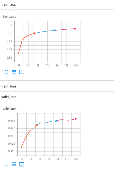
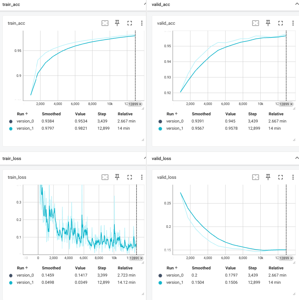
3) 신경망의 훈련예제에서 훈련/검증 손실과 정확도를 텐서보드를 이용하여 그래프로 그려보라.
- 매 에퍽마다 실시간으로 그래프를 업데이트하도록 할것 -> 훈련동안 시간의 흐름에 따라 loss의 변화를 확인가능하도록 할것
1 2 3 4 5 6 7 8 9 10 11 12 13 14 15 16 17 18 19 20 21 22 23 24 25 26 27 28 29 30 31 32 33 34 35 36 37 38 39 40 41 42 43 44 45 46 47 48 49 50 51 52 53 54 55 56 57 58 59 60 61 62 63 64 65 66 67 68 69 70 71 72 73 74 75 76 77 78 79 80 81 82 83 84 85 86 87 88 89 90 91 92 93 94 95 96 97 98 99 100 101 102 103 104 105 106 107 108 109 110 111 112 113 114 115 116 117 118 119 120 121 122 123 124 125 126 127 128 129 130 131 132 133 134 135 136 137 138 139 140 141 142 | import torch import pytorch_lightning as pl import torch.nn as nn from torchmetrics import Accuracy from torch.utils.data import DataLoader from torch.utils.data import random_split from torchvision.datasets import MNIST from torchvision import transforms from pytorch_lightning.callbacks import ModelCheckpoint class MultiLayerPerceptron(pl.LightningModule): def __init__(self, image_shape=(1, 28, 28), hidden_units=(31, 26)): super().__init__() self.train_acc = Accuracy(task="multiclass", num_classes=10) # 정확도 속성 -> 훈련 중에 정확도를 추적할 수 있음 self.valid_acc = Accuracy(task="multiclass", num_classes=10) # torchmetrics에 속함 self.test_acc = Accuracy(task="multiclass", num_classes=10) input_size = image_shape[0] * image_shape[1] * image_shape[2] all_layers = [nn.Flatten()] for hidden_unit in hidden_units: layer = nn.Linear(input_size, hidden_unit) all_layers.append(layer) all_layers.append(nn.ReLU()) input_size = hidden_unit all_layers.append(nn.Linear(hidden_units[-1], 10)) self.model = nn.Sequential(*all_layers) def forward(self, x): # 입력 데이터로 모델을 호출할 때 마지막 완전 연결층의 출력을 반환하는 계산 수행 x = self.model(x) return x def training_step(self, batch, batch_idx): x, y = batch logits = self(x) loss = nn.functional.cross_entropy(self(x), y) preds = torch.argmax(logits, dim=1) # 줄일 차원 1 self.train_acc.update(preds, y) self.log("train_loss", loss, prog_bar=True) return loss def on_train_epoch_end(self): self.log("train_acc", self.train_acc.compute()) self.train_acc.reset() def validation_step(self, batch, batch_idx): x, y = batch logits = self(x) loss = nn.functional.cross_entropy(self(x), y) preds = torch.argmax(logits, dim=1) self.valid_acc.update(preds, y) self.log("valid_loss", loss, prog_bar=True) return loss def on_validation_epoch_end(self): self.log("valid_acc", self.valid_acc.compute(), prog_bar=True) self.valid_acc.reset() def test_step(self, batch, batch_idx): x, y = batch logits = self(x) loss = nn.functional.cross_entropy(self(x), y) preds = torch.argmax(logits, dim=1) self.test_acc.update(preds, y) self.log("test_loss", loss, prog_bar=True) self.log("test_acc", self.test_acc.compute(), prog_bar=True) return loss def configure_optimizers(self): optimizer = torch.optim.Adam(self.parameters(), lr=0.001) return optimizer class MnistDataModule(pl.LightningDataModule): def __init__(self, data_path='./'): super().__init__() self.data_path = data_path self.transform = transforms.Compose([transforms.ToTensor()]) def prepare_data(self): MNIST(root=self.data_path, download=True) def setup(self, stage=None): mnist_all = MNIST( root=self.data_path, train=True, transform=self.transform, download=False ) self.train, self.val = random_split( mnist_all, [55000, 5000], generator=torch.Generator().manual_seed(1) ) self.test = MNIST( root=self.data_path, train=False, transform=self.transform, download=False ) def train_dataloader(self): return DataLoader(self.train, batch_size=64, num_workers=4) def val_dataloader(self): return DataLoader(self.val, batch_size=64, num_workers=4) def test_dataloader(self): return DataLoader(self.test, batch_size=64, num_workers=4) import torch.multiprocessing if __name__=='__main__': # 오류땜에 추가 import os log_dir = './lightning_logs' if os.path.exists(log_dir) and not os.path.isdir(log_dir): os.remove(log_dir) # 기존 파일 삭제 os.makedirs(log_dir, exist_ok=True) # 디렉토리 생성 torch.multiprocessing.freeze_support() torch.manual_seed(1) mnist_dm = MnistDataModule() mnistclassifier = MultiLayerPerceptron() callbacks = [ModelCheckpoint(save_top_k=1, mode='max', monitor="valid_acc")] if torch.cuda.is_available(): # if you have GPUs trainer = pl.Trainer(max_epochs=15, callbacks=callbacks, gpus=1) else: trainer = pl.Trainer(max_epochs=15, callbacks=callbacks) trainer.fit(model=mnistclassifier, datamodule=mnist_dm) | cs |
4) 신경망을 구현할때 사용하는 파이토치 클래스를 모두 설명하라.
- torch.nn.Module : 파이토치의 모든 신경망을 정의할 때 상속받는 기본 클래스
- torch.nn.Linear : 선형 변환을 수행하는 계층. 입력 크기와 출력 크기를 지정하여 완전 연결된 신경망을 구성할 때 사용
- torch.nn.ReLU : ReLU 활성화 함수. 음수 값은 0으로 처리하고 양수 값은 그대로 전달하는 비선형 함수
- torch.nn.Sigmoid : Sigmoid 활성화 함수. 출력값을 0과 1 사이로 압축하는 함수
- torch.nn.ModuleList : Module을 여러 개 리스트 형식으로 저장하는 클래스
- torch.nn.Sequential : 여러 Module드을 순차적으로 쌓을 때 사용하는 클래스
5) 신경망 모델의 입력텐서의 원소는 [0,1]사이로 정규화 하는 이유를 설명하라.
- 입력텐서의 원소를 [0,1]사이로 정규화 하는 이유는 입력 값의 범위가 너무 크거나 작으면 신경망의 역전파 과정에서 발생하는 그레이디언트가 너무 커지거나 작아져서 학습이 불안정해질 수 있기 때문이다.
6) 신경망 모델의 출력값의 범위에 대하여 설명하라.
- 신경망 모델의 출력값의 범위는 모델의 목적에 따라 달라진다. => 주로 문제의 종류와 활성화 함수에 의해 결정됨.
(1) 이진 분류
---> 출력값 : [0,1] 사이의 값 (시그모이드 활성화 함수가 출력값을 0과 1 사이로 변환하여 클래스 확률을 제공함)
(2) 다중 클래스 분류
---> 출력값 : [0,1] 사이의 값 (소프트맥스 활성화 함수가 각 클래스에 대한 확률을 계산하며 출력값의 합이 1이 되도록 반환함)
(3) 회귀
---> 출력값 : 실수(제한 없음) (선형 활성화 함수 사용. 출력값이 범위 제한 없이 자유롭게 변화할 수 있도록 함)
(4) 이미지 생성
---> 출력값 : 이미지 픽셀 값은 [0,1] 범위로 정규화 되거나 [-1,1] 범위로 정규화 되기도 함.